The Misuse of Correlation Part 4

Continuing from the previous post, I’m looking at issues and common mistakes arising from the use of the word correlation.

1. Uncorrelated does not mean unrelated
2. Correlation does not imply causation
3. Correlation is not transitive
4. Data issues

We have covered number 1 and 2 already.

3. Correlation is not transitive.

In my post on significance, we covered that only some relationships are transitive.
For example, weight is a simple example of a transitive relationship

• If Adam weighs more than Bert
• And if Bert weighs more than Charlie
• then Adam weighs more than Charlie.

But, just as for significance, this is not true for correlation.

Modern medicine gives us many clear examples

• High cholesterol correlates with higher risk heart disease
• Certain drugs (e.g. statins) correlate to lower cholesterol
  Therefore

• Certain drugs (e.g. statins) correlate with lower risk of heart disease

Correlation is not transitive so this is a common logic error.
We have to study the direct relationship of the drug and heart disease to see. But by the time the statins advice was given, trials were still not conclusive. Respecting this problem makes proper drug testing expensive and difficult, but ignoring it, makes writing an article in the Daily Mail really easy.

I saw a similar result in the news recently.

• Taking aspirin correlates to lower risk of heart attack
• Heart attack correlates to early death
  Therefore

• Taking aspirin correlates to lower risk of early death
  However, having trialled this with real patients, the results found
• Taking aspirin also correlated to fatal internal bleeds (especially in the elderly)

Doctors are now much less confident in their original advice as the number of deaths, due to taking are thought to be material, so other factors must be considered.

Not only is this relationship non-transitive, but it’s clear how complicated the real world and overly simple results from correlation may be very misleading.

Similar examples we see in financial markets.
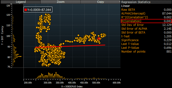
Let’s build a basic model for the oil price using two drivers, inventories, and the US dollar. If I run a regression of the over 10 years, I get a correlation coefficient:

• –0.78 for the oil price and the level of inventories
• –0.44 for the oil price and the US dollar.

What do I get if I do a regression of oil inventories and the US dollar?

• 0.04 i.e. virtually no correlation at all.

4. Data issues

A. The problem of selective attention

“How not to be wrong” by Jordan Ellenberg mentions this good example of Berkson’s fallacy.

“Why do literary snobs believe that popular books are badly written?”

• Let’s imagine a world in which half the books are popular and half the books are unpopular.
• Only 20% of the books are good with 80% being bad.
• Let’s make no relationship (correlation) between those two variables.

We would get the grid below:

However, who pays attention to books which are both bad and unpopular?
No one

From a literary snob’s point of view, you can redraw the grid with only the books they are conscious of existing (i.e. the unpopular bad books are in a blind spot)

The grid they perceive looks like this:

In this case, they see the important statistics as

• Half of good books are unpopular (10/20)
• 80% of popular books are bad (40/50).
• A bad book has a 100% chance (!!) of being popular (40/40)

Conclusion “people have terrible taste and to make some money I should write a bad book!”

Given the perceived data set, this conclusion would be solid. But looking at the entire data set, it’s clear that they are making a mistake.

We are in danger of doing this all the time in economics and finance. But finding a good example is hard as the whole point of a blind spot is that we tend to be unaware of it.
What is clear is that the choice of data set is critically important, and likely a far more important choice than the sophistication of the statistical tools you later apply.

B. Choosing a time window

A related and common problem in financial markets analysis is the biased selection of data.
As I wrote about more fully in Significance (https://appliedmacro.com/2017/06/12/the-misuse-of-significance/), analysts often want to produce statistics with compelling results.

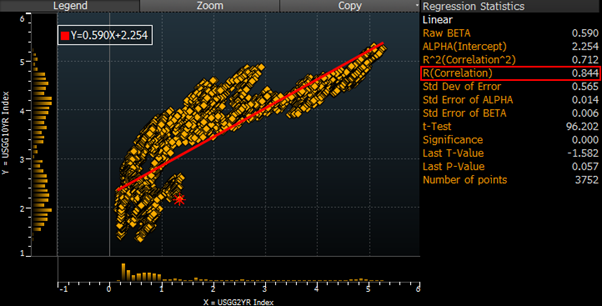
For correlation type analysis, the most common trick is the selection of the time window. If we take the short and long-term interest rate example from Part 1 “Uncorrelated does not mean unrelated.” We observed that the correlation is very close to zero for the last 5 years. However, if we extend the time window to the last 15 years, the correlation increases dramatically to 0.84 which is a decent relationship.

Conclusion

In these posts, I have discussed a number of ways in which correlation analysis is misunderstood and misused. Analysts often know these issues, but they still manage to fall into the traps. I have certainly been guilty of making all the mistakes above many times! I have tried hard to train my analysts to watch out for this sort of error in their work and encourage them to look for it in the work of others – it can be hard to spot once you’ve already worked hard on something.

Of course, these are not the only errors made with correlation in finance. The more serious mistakes follow from a more profound misunderstanding of correlation which took me many years and a lot of painful experiences to gain an appreciation of. I will turn to those in the next post.