In this post, I want to talk about an insidious error that creeps in with the usage of correlation in finance.
FT lexicon supports the idea that:
“a correlation is said to be positive if movements between the two variables are in the same direction and negative if it moves in the opposite direction.”
This definition is not unusual, commonly seen in finance textbooks.
Occasionally the formula may be presented:
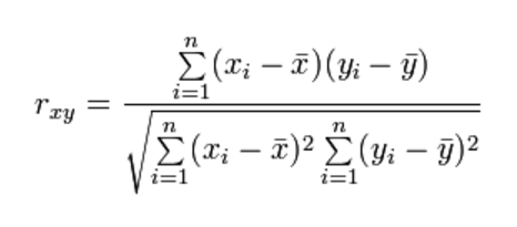
But caveats in using the formula will likely be absent or at the least hidden from view.
By that, I mean the terms  and
and  are critically important but this importance is rarely appreciated. [1]
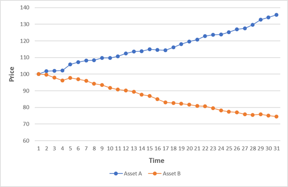
In the previous post, I asked you about the correlation of the changes of the two assets in the chart below:
a. Positive correlation
b. Negative correlation
c. They are uncorrelated
d. Not sure (be honest!)
The most obvious answer is of course b)
One line goes up and the other goes down so this means they have a negative correlation. This is unfortunately strictly incorrect if you paid attention to the instruction to consider the “changes in the two assets”.
A good answer is d)
Given the amount of information I had supplied, it’s a perfectly reasonable one.
Because another answer is a)
The correlation of the changes in the variables is +1, PERFECT POSITIVE correlation
and the lines are going in the OPPOSITE direction!!
(If you doubt this result please look at the data and calculations in the sheet attached (download) and use the CORREL function in excel.)
b) is an intuitive answer but a) is the answer that a financial analyst would calculate. If you imagine of situations where you are being given financial advice, it is clear there could be an immediate conflict!
First insidious confusion – the importance of the mean
If you have never seen this before, you may think I am lying or this is a convoluted trick. But it rests upon one key part of the calculation of correlation that is missing from virtually every definition I see, and is certainly missing from the vast bulk of work done by analysts in the finance industry.
The key is that correlation is calculated by looking at the relationship in deviations from the means (the terms and in the complicated mathematical equation).
In our example, the changes in the two variables in the chart have equal and opposite means, and so trend in different directions. However, the day to day volatility (deviation from the mean of the changes) is identical for both variables, and it is this term that drives the correlation whilst having no impact on the trend.
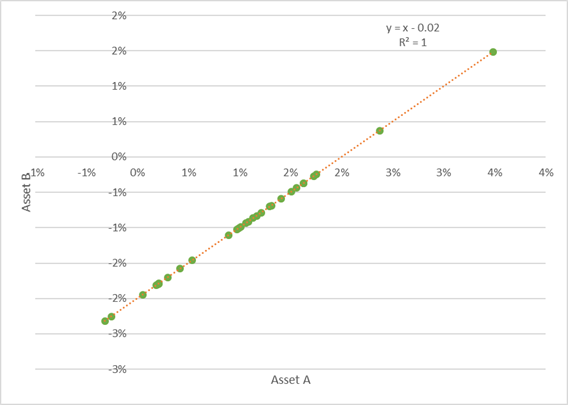
Here is a scatterplot of the % changes for each variable. Observe all the dots are distributed along the line – a perfect POSITIVE correlation.
This has a clear relationship to the way we think about the change in market prices of any asset:

In financial markets, the daily noise is usually much greater than the daily trend, and so forms the focus of most market commentary.
The key result is that if the noise term correlates for two assets, then they will correlate irrespective of their underlying trend, given the way correlation is calculated.
i.e. they could end up in very different places even if they are positively correlated!
Second insidious confusion – levels vs changes
The second insidious confusion can arise from a reference to correlation of the CHANGES or a correlation in the LEVELS of the two variables.
In financial markets, the method invariably used is to look at the changes in variables. In our example, we get the answer of positive 1 i.e. perfect positive correlation.
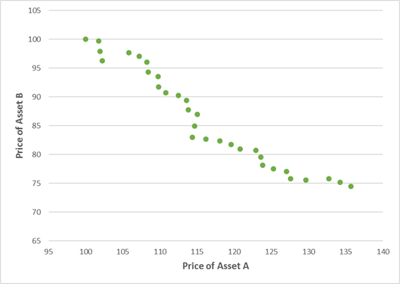
If we calculate the correlation using the levels or prices, we get an answer of -0.97
i.e. strong negative correlation
The intuitive result is the opposite of the result most likely to be calcuated by financial analysts.

Why does finance prefer the use the correlation of changes?
It is done for good reason. When you are looking at data with strong trends, as a lot of asset prices do, the correlation of levels can yield very strange results. Let’s take an example.
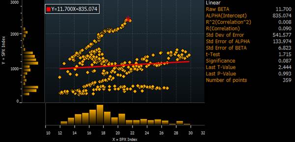
Let’s look at the US equity market (S&P 500 price – white line) and its PE ratio (orange line) over the last 30 years.

If we first look at the correlation of levels, we get a correlation of virtually zero.
This suggests a rather unintuitive result that there is no meaningful correlation between PE ratio and equity prices!
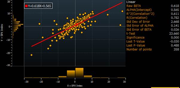
If we instead look at the correlation of changes, we get that there is a meaningful positive correlation of 0.78 which makes a lot more sense.
Conclusion
If these differences in the correlation results is were just some statistical fluke, from a couple of silly examples, then it would not matter.
But it is not an unusual result and it occurs when looking at the biggest and most commonly traded financial markets. It is therefore critical to avoid confusions such as these when thinking about what type of correlation to use or, more often, what someone else has used in the analysis you are reading.
[1] I very much enjoyed this paper by Francois-Serge Lhabitant which explains this issue very well. http://www.edhec-risk.com/edhec_publications/all_publications/RISKReview.2011-09-07.3757/attachments/EDHEC_Working_Paper_Correlation_vs_Trends_F.pdf