Can you put a price on the environment?

I am an economist by training, experience and by inclination so the answer seems an obvious yes. Welfare economics generally looks at exactly these sorts of questions. However, the debate and current policy mix for Climate Change does not appear how I would expect it to, especially given the lack of agreement on carbon pricing which has dropped out of the discussion.


Assigning monetary value?

A common mistake that economists make is, because a given model works for some aspects of human behaviour, they assume it can always be used and possibly generalised to all human behaviours, often by adding some sort of arbitrary assumption to make it fit. The consensus in neoclassical modelling is for a marginalist approach with rational agents.

Take gift giving, it is economically inefficient but still takes place. The neoclassical approach is to assume that cash giving has an unexplained stigma or that buying your lover a thoughtful gift acts as signal that you love them. Of course, these fail to resonate with our actual experience of gift giving and receiving, and so fail the common-sense approach.

This is a classic logic error – there are many (infinite?) ways to model and explain behaviour. Just because you have one that you like does not mean it is the only one or that it must be superior to the others. If to make your model fit the external reality you are required to add counterintuitive assumptions then this can often sign to rethink your entire approach.


What other approaches are there?

The environment is a moral not an economic question

This idea was sparked reading Michael Sandel’s “What Money Can’t Buy”.
As a political philosopher, he is highly critical of the current trend towards adding commercial thinking and monetary values into our lives, using moral arguments of unfairness and degradation of values. There are many examples: paying to avoid queuing, the rise of corporate boxes at venues, paying to get a nicer prison cell and, in this category, he also places the environment.

Another famous example of a counterproductive effect of replacing a moral code with a monetary incentive is a school adding a fee for late pick-up of children after school. Parents were much happier paying a price for lateness than infringe a moral obligation to pick up the children on time and the incidence increased. Related to this, when people are paid for blood donations, the amounts and quality of blood donated both fall.

When Sandel in 1997 wrote a piece in the New York Times arguing against carbon trading, he was inundated with “scathing letters – mostly from economists” who assumed that he simply did not understand that their model, that trading would always be good, was obviously true. 20 years later some economists may be more sympathetic to the idea that not everything should be analysed in this way. http://www.nytimes.com/2011/04/22/opinion/22krugman.html?_r=1&hp

A different view?

Do the efforts to “stigmatize” excessive carbon usage and “promoting virtuous attitudes” work? Moral codes in society are very powerful. But as a prevention mechanism, they do not always work. They may not be as universally shared as their advocates like to assume; If you want to reduce teen pregnancy the approach of teaching that sex before marriage is immoral and the promotion of abstinence have been shown to be highly ineffective. The attempt to change people’s behaviour on carbon consumption by stigmatizing it appears to me to have the same flaw. People may feel a little guilty but will not actually change their behaviour, whilst the moralisers can enjoy the feeling of superiority, getting us nowhere.

I was once memorably informed that my willingness to experiment with models and analysis that put a monetary value on human life was “sociopathic”. I did wonder at the time if they knew or cared how counterproductive it is to alienate sympathetic non-believers if your objective is to influence behaviour.


Lexicographic vs marginal preferences

Amartya Sen is a wonderful writer on justice, development and social choice who developed ideas in welfare economics beyond thinking purely about Pareto optimality. I was recently reminded of this concept in Marc Lavoie’s “Introduction to Post-Keynesian Economics”. It was striking to me that I had forgotten about it which implies it is not commonly used.

Faced with needs, the idea is that people do not make marginal decisions across every item but rather make choices only within categories. There is a hierarchy of needs, and only when the essential ones are obtained, then the next category can be bought. Therefore, substitution of goods only happens within categories and not between them.

For the environment, people that think that climate change is a compelling moral issue then discussing the price is bizarre and inappropriate. It is a moral need and comes in a very important category. For people who have consumption desires they find more pressing such as housing, clothing and food, then the morality of climate change is in a lower category and so not highly valued. This helps explain the observation that when asked how much they value the environment people’s answers tend to be extremely high numbers or extremely low ones. There is no smooth substitution along an indifference curve. It also explains why people express that they care enormously about the environment when the economy is doing well and it is not mentioned during a recession.

This sort of heterodox critique of neoclassical marginalism is compelling, but the next step of suggesting a policy is lacking. Lavoie says that “post-Keynesians have never really developed their views on consumer choice in any systematic way” and only have “insights”.

Where next?

I am left thinking that at pure moral non-market approach to dealing with Climate Change is not effective. A lexicographic approach gives a useful description that fits observed behaviour but does not give me any useful approaches to designing policy. So, I return to welfare economics and thinking in terms of cost-benefit analysis and externalities.

Framework for valuing equities Part I- Compared to bonds

A useful framework for considering one investment is to compare it with another, you can then do analysis to decide if you prefer one to the other. This is of course relative value and if the benchmark asset is government debt, this is a solid place to start.

The “Fed Model”

The “Fed Model” is that the stock market yield is related to the yield on long-term government bonds. Like so many models, it has fallen into disrepute seems to come more from its misuse over the years as opposed to its intrinsic failings.

Expected Returns for Equities and Bonds

A way to start thinking about this model is to start with the expected returns on the two investments, equities and bonds. Consideration of the spread of returns and the distribution around the expected return can come later.


Bonds

Expected return for US government bonds in nominal terms is as easy as it gets – yield to maturity.
I will ignore the remote possibility of a default on the debt.

Equities
Expected returns for equities is harder; there is a choice of possible yields, with none necessarily equating to the eventual return.

  • Dividend yield
    Problematic given that dividend policy is a management decision. Microsoft’s decision not to issue dividends was not a good indicator of its total return.
  • Earnings yield
    More sensible i.e. E/P (or just PE ratio inverted).
  • Earnings yield + Inflation

Considering we are using historical earnings, to get a future value we could add an inflation component given that earnings would be expected to rise along with inflation, in the long run.

Testing the expected returns model for Equities

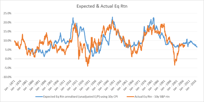
Back-testing expected returns to 10 year actual returns, the US equity market shows surprisingly good results, especially post WW2. This makes intuitive sense as one would expect that buying equities with a lower PE or when inflation is higher would produce better returns. But the strength of the relationship is eye-catching, implying that current earnings do on average provide a good guide to expected equity total returns.

If you come from a purely “efficient markets” view of the world, this may seem blindingly obvious with equity value as simply the present value of the earnings stream. But bear in mind that earnings yield (E/P) is not a yield in the same way that bonds have a yield, unless you make an argument where the word “assume” occurs very frequently.


Expected Returns for Equities versus Bonds

Given that we are happy with our model of expected returns for both equities and bonds, we can move on to comparing one versus the other.

The model for expected return of equities over bonds would look like

We can use data from end 2016 to get actual numbers

This difference/expected return is often called an equity risk premium (ERP).

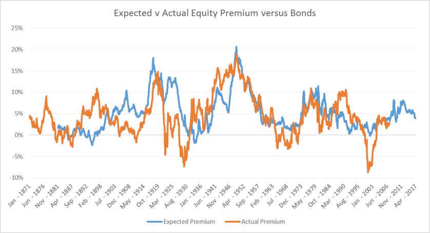
We can now back-test its use in predicting if the equity market will actually outperform the bond market. Chart below again shows pretty decent relationship – but can we say how good?

expected vs actual

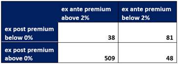
Given the nature of the data we should not perform a regression, and instead here is a truth table for the data back to 1950.

With ex ante premium (i.e. model) above 2%, then equities outperform bonds 93% of the time.
With it below 2%, then equities only outperform 37% of the time. That is a pretty solid result.

Summary

This investigation that equities look cheaper than bonds. If this is the only model you use then the clear imperative is to buy equities now. Before I make my mind up, I want to think about fixed income valuation next.


Government Debt Framework – UK Follow-up

Relevance to the present

Previously, we looked at the UK government debt in the post WW2 period.

Two clear questions arise –

“How did the UK manage to keep its rates so far below nominal GDP?”
“Should we expect to be able to do the same in the future? “

The key to inflating away national debt is the ability to force domestic investors to hold government debt at well below the yield they would get in a free price-setting environment.
Sometimes this is reported as financial repression.

Again, this paper does a really good job of giving the details of the post WW2 period. https://www.imf.org/external/np/seminars/eng/2011/res2/pdf/crbs.pdf

Comparison post WW2 period to Current

I am interested in the extent to which the situation could be the same for other countries today.
My bias is that it would be significantly more difficult and we should not assume that because it worked in the 1950s it will work today.

  1. Ability to force domestics to hold govt debt
    This is probably the easiest and we are seeing plenty of this at the moment.
    e.g. pension funds and banks being required to hold government debt for “liquidity” or “prudence”

But the danger of the current system is leakages

  1. Capital controls
    Post war Bretton Woods we had globally imposed coordinated capital controls that reinforced home bias. In effect, countries agreed not to compete for capital through the price mechanism. I see this as a form of cartel which managed to hold together until the 1970s. We are a long way from that kind of cooperation today.
  1. Ownership of debt
    It is much easier to coerce domestic investors than foreign ones. In many heavily indebted countries, the issue is that debt markets are owned by foreign investors. This was a big factor in the Asian crisis of 1997/8 and the Mexico crisis of 1994. Currently, the Gilt market is 25% owned by overseas investors which makes it perhaps a little vulnerable. In contrast Japan has a higher debt level but virtually all the debt is owned by domestics.
  1. Trade surplus/deficit
    Post WW2, the UK was close to balance and now has a large deficit (over 4%). This deficit needs external funding which currently comes from FDI. All this adds extra pressure and vulnerability to the situation.
  1. Sensitivity of average rate on the of debt
    In ideal world, the debt market would be structured as conventional Gilts with as long tenor as possible whilst running a primary surplus to offset the interest payments. Even if short rates and inflation rose, the rate paid on the debt would stay the same thus somewhat mitigating rollover risk or the risk of paying much higher rates overall. Unfortunately, this is not the case in most developed countries as QE has been making situation worse.

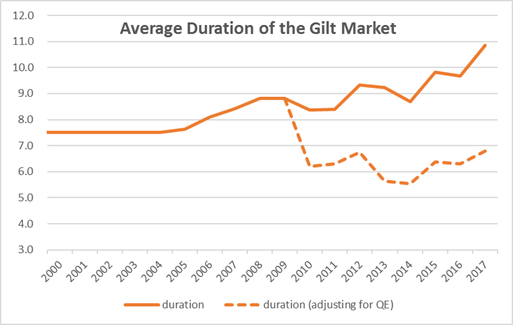
QE shortens duration of the debt market

One way to think of QE is as a shortening of the duration of debt issuance (another post I think) then the impact on the debt profile is to significantly shorten it. In this light, QE on the Bank of England’s balance sheet simply means that rather than having a £435bn liability of long duration it is paying overnight rates on bank reserves. When (/if?) the Bank raise rates then they are immediately paying higher rates on the debt. (note debt and liability mean the same thing here).

Below is a chart of the average duration of the Gilt Market since 2000

image0011


Final Thoughts

I have frequently read the argument that we can inflate our way out of our current debt problems by having faster growth and inflation. The obvious flaw in this argument is it requires independence of nominal GDP growth and interest (i.e. Central Banks would not raise rates in the face of higher nominal growth which is clearly not the case). In the modern market economy, nominal growth and interest rates are highly related and so just assuming they are not is both bizarre and surprisingly common. Alternatively, you can concede that there is a link between growth and interest rates but remain very confident in the ability of modern nation states to impose financial repression with no leakages.

From my understanding of the modern financial system, I do not share that confidence that current debt levels can be easily reduced and therefore, I do not think they can be raised with impunity. It does not however follow that I become an austerity-hungry debt and deficit hawk.

This debate that I read between economists and political commentators appears depressingly partisan with far more noise and anger than analysis. What really matters is whether the current situation is risky enough to merit policy action or, as investors, some active asset re-allocation. This is highly complex but in my view, economic analysis is falling short in its ability to help. If your answer to the question of whether government deficits should be higher or lower is the same at all times, across all countries, then I would suspect that your economic model is not going to be very helpful in making policy or investment choices.

Government Debt Framework – UK

Introduction

For anyone interested in the long-term investment outlook for fixed income, or more simply the future of our current sovereign nation states, an understanding of government debt must be a key element. Much is written on this subject but I find a lot of it confusing with partisan politics dominating analytical perspectives and terminology which is often inconsistent and emotive.

In this note, I want to focus on episodes where large debt level has been managed.
The large debts of WW1 and the Great Depression were reduced, on the whole, by various types of default. These always come with large economic costs and are to be avoided.
The period after WW2 is more interesting, commonly used as evidence as grounds for optimism and as grounds for opposing “austerity”. (in quotes as this term is generally emotively used by the opponents of current fiscal policy and has a pretty loose definition and usage)

(This paper by Reinhart and Sbrancia does a nice job of laying out the economic history. https://www.imf.org/external/np/seminars/eng/2011/res2/pdf/crbs.pdf)


Government Debt Model

So, I thought I would start by making a simple framework within which I can look at debt dynamics. Breaking down the change in government debt into 2 parts:

  1. Primary surplus
  2. Interest payments

(put simply Overall Deficit = Primary deficit + interest paid)

Note, this is not intended to be a complete model as there are clearly other factors which can change the debt level. For example

  • Change in currency level for foreign-denominated debt
  • Change in yields leading to change in market value of the debt
  • Due to Extraordinary items e.g. the government takes on additional debt which for accounting reasons they do not show up in the primary deficit

But it is pretty decent and captures the vast majority of the debt dynamics, certainly all of the ones which drive long-term trends.


Model UK Gilt History

Here is the model vs actual data since WW2 for the UK.
image001

There are two clear episodes (~1974 and ~2008) when the actual increase in government debt were far larger than the model would suggest. It would be nice to understand what drove it (for example, in the financial crisis, did the government balance sheet absorb private sector banking debt without having it showing up in the deficit?)

Below is the chart of UK debt since WW2

image002

It is commonly described that the UK ran deficits thought this period and the debt level was brought down by high growth. This is not incorrect but I find it a bit narrow and misleading.

Budget Deficit v Primary Deficit

First, the idea that the UK ran deficits. Well it is true but if you split the deficit into primary surplus/deficit and interest payments then the picture looks quite different.

image003

During the 1950s and 60s, the UK run a deficit virtually every year. But we can also see that the UK ran a primary surplus for the entire period. So the reason the UK ran a deficit was simply that the debt levels were very large and so the interest payments were very large.

Whilst it is true that the main way the UK brought down its debts level was running nominal GDP at a higher rate than the interest rate paid on its debt, compounding effects are huge (running this for a long time) particularly when the debt level is large.

Between 1947 and 1951, debt levels fell from 246% to 165% of GDP. The cumulative primary surplus over that period was 29%, so the balance, about 2/3, of fall in level came from the impact of nominal GDP vs the rate on the debt. compared with only 1/3 from running large primary surpluses.

image004

Relevance to the present

How did the UK manage to keep its rates so far below nominal GDP?
Should we expect to be able to do the same in the future?