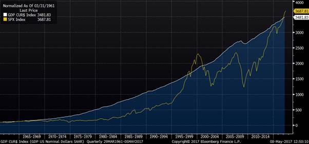
We explored in the last post (Framework for Equity Valuation Part II – Equity Drivers) how earnings as a share of GDP can be an important driver of medium term equity returns.
What is the market expecting earnings to be?
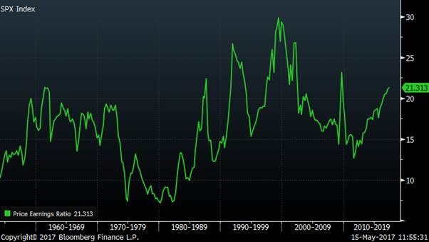
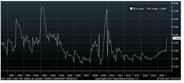
The chart below shows the difference between what the PE ratio is today and what it is expected to be in a year’s time (i.e. a measure of what analysts expect total earnings growth to be). Currently it shows that equity analysts are predicting a 20% increase in corporate profits. This implies that although the current PE ratio may be high, it will be brought down by rapidly rising earnings.
I find this chart is the best explanation of the Trump rally. Analyst earnings expectations rose immediately and this is temporarily reflected in a higher PE ratio. Once the earnings come through we will see that the rise in equities was driven by earnings not by animal spirits. Assuming the analysts’ earnings optimism is correct of course.
What does this mean for earnings over GDP?
I will leave aside for now views on how effective Trump will be at increasing growth and just look at the confidence level implied in market prices. It is all too easy with controversial political figures and issues for analysis to become infected with partisan assumptions and desires which lead to worse decisions.
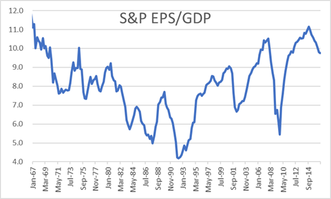
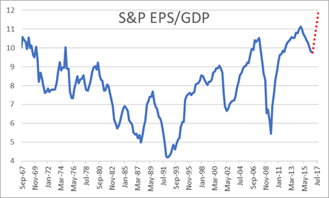
The first point to note is that taking analysts expectations of a 20% earnings increase, this would imply earnings as a share of GDP will immediately rebound to all-time highs (dotted red line in the chart we used previously). We have seen drops in E/GDP of that magnitude before during recessions but never an increase and this seems an odd stage of the cycle to expect it.
Is this forecast consistent with other data?
Another useful way to use national income data is split the economy into just 2 parts – Wages and Profits.
The National Income Accounts (NIPA) data is used a lot more by economists than it is by market participants. To give some context, it was particularly useful to use during the late stages of the dot com bubble, as it showed that reported earnings were far in excess of the profits seen in the national accounts. This implied some form of earnings inflation and potentially even fraud, which actually did come to light later in 2002. The chart below shows how the reported earnings diverged for 4 years before coming back in line very sharply. Checking reported data and forecasts for simple internal consistency can be surprisingly rewarding. It is best not to assume that analysts have done this for you.

Using the National Income Accounts data, we can construct a chart of the respective shares of national income for wages and profits. As you can see, there is a clear and logical inverse relationship between wages and profits as a share of GDP.
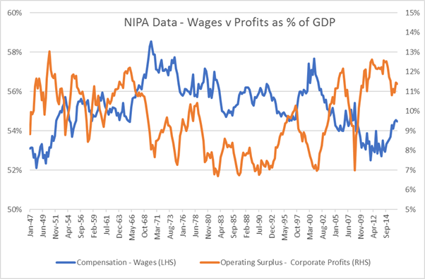
We know that wages have finally been rising again recently and all forecasts are that this will continue. So how can we have nominal GDP of 4%, wages rising at least 2.5% and profits rising 20%.
Quick answer – we can’t.
Long answer – it requires some heroic assumptions in other parts of the national accounts which I won’t go into here.
Scenario – if we assume corporate earnings will rise by 20% over the next 12 months and allow the other components of GDP (including proprietors’ income) to grow at 4%, we can solve for wages and we get an increase of just 0.7%. Rather different from the 2.5% current seen in average hourly earnings.
Summary
There is a great deal of optimism among analysts for the outlook of corporate earnings. It is hard to reconcile that with some basic arithmetic from the national accounts. When nominal GDP growth is moderate and wages are accelerating, it is hard to also get record increases in corporate profits. If earnings do not rise as rapidly as anticipated then to be optimistic on the S+P you need to be positive on the prospects for PE expansion. I will look at that next.