In the beginning, there were people….
People have social interactions which have very strong patterns. One of these patterns is the concept of Reciprocity. If someone gives you something you have a strong sense of obligation to give them something back. This forms the basis on many successful marketing strategies (see “Influence” by Robert Cialdini) but also sits at the heart of everyday social interactions.
For example, in the office someone makes coffee for you. This creates an implicit obligation which you will wish to later reciprocate, or perhaps “repay”. In fact, the word “pay” is said to come from Latin “pacare” meaning “to pacify” and later came to mean to settle a debt. You do not immediately barter, need to give something in return at that time. You have a social relationship and there is mutual trust that this obligation will be repaid. This obligation could be called a “debt” or a “liability”. The person who made the coffee now can be seen to be holding an “asset”.
Make it more useful by adding features….
This method of economic organisation works well for small items between tight-knit or homogenous groups. But it would be far more powerful if we could add some other features which allow us to expand it:
- Unit of measurement.
It is handy to be able to quantify the economic value of the transaction so that more complex exchanges can be facilitated - A method of recording ledger items.
Just remembering that it is your turn to buy doughnuts for office is not sustainable for more complex economic transactions. - Tradability to a 3rd party
It would be great to be able to have the favour repaid by someone other than the recipient.
A voucher system….
So let’s start a voucher system. Every time you do me a favour such as babysit my kids I will give you a voucher. Every time I do a favour such as mow someone’s lawn I will be given a voucher. I can build up a stack of voucher from doing these jobs and then “spend” them by taking my family to a restaurant for dinner.
This system of money can be seen today in small areas. In the UK, there is the Lewes pound and the Brixton pound. Tight-knit communities can develop all sorts of formal and informal social conventions to regulate exchange. None of them require gold. These are the sorts of systems of money found in ancient, primitive societies. There is no strong archaeological evidence because this kind of money is not physical, however the earliest writing ever discovered was on tablets thought to represent ledger type records. Tokens in the form of Coins are in fact a later discovery and this has commonly been misunderstood as thinking that it was the tokens themselves that were the valuable item. In fact, it was and is the social obligation that matters, coins were simply a means of recording it.
Using a central authority to widen the usage….
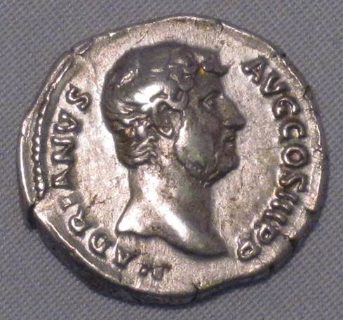
But these local currencies or voucher systems have limitations. They rely on trust which is hard to foster with strangers. It would be much more powerful to have some authority or government to issue the money and guarantee its use across a broader area. This is when we see minted coins by a sovereign.
The unit of value can be solidified by collecting taxes in that unit. You will notice that you owe your taxes in US dollars in the US, and in pounds sterling in the UK. The benefit to society is huge, economic activity can be distributed and exchange facilitated on a grand scale. There is also a large benefit to the government, as issuer they get to earn seignorage.
Conclusion
The alternative story of money is still taught, but these days it is mainly in sociology, history or anthropology departments. This version has been eradicated from economics faculties and treated as “fake news”. Economics students are not taught arguments to support their story, it is simply assumed and most are even unaware there are other ideas.